Assesses confounder balancing

Draws on functions from the cobalt package to quantify the relations between exposure and confounders at each exposure time point according to the guidelines from Jackson, 2016 on how to assess balance for time-varying exposures.

Usage

assessBalance(
  data,
  obj,
  weights = NULL,
  balance_thresh = NULL,
  imp_conf = NULL,
  verbose = FALSE,
  save.out = FALSE
)

# S3 method for class 'devMSM_bal_stats'
print(x, i = NA, t = TRUE, save.out = FALSE, ...)

# S3 method for class 'devMSM_bal_stats'
summary(object, i = NA, save.out = FALSE, ...)

# S3 method for class 'devMSM_bal_stats'
plot(x, i = NA, t = TRUE, save.out = FALSE, ...)

Arguments

data

data in wide format as: a data frame, list of imputed data frames, or mids object from the mice package

obj

initialized MSM object from initMSM()

weights

(optional) list of IPTW weights output from createWeights()

balance_thresh

(optional) one or two numbers between 0 and 1 indicating a single balancing threshold or thresholds for more and less important confounders, respectively (default = 0.1)

imp_conf

(optional) list of variable names reflecting important confounders, required if two balance thresholds are supplied

verbose

(optional) TRUE or FALSE indicator for printing output to console. default is FALSE.

save.out

(optional) Either logical or a character string. If TRUE, it will output the result to a default file name within home_dir set in initMSM(). You can load the data with x <- readRDS(file). To use a non-default file name, specify a character string with the file name. It will save relative to home_dir. There might be naming conflicts where two objects get saved to the same file. In these cases, users should specify a custom name. default is FALSE.

x

devMSM_bal_stats object from assessBalance

i

For multiply imputed datasets, i selects which imputation to print results for. Default is i = 1. With i = TRUE, all imputed datasets will be looped over. With i = NULL, will average over all imputed datasets and summarize that. Ignored for non-imputed data.

t

Which exposure variable to use. Can either be an index from 1 to the number of exposures or a string containing the exposure variable name (e.g. "A.3"). With t = TRUE, all exposure variables will be looped over.

...

ignored

object

devMSM_bal_stats object from assessBalance()

Value

a list containing balance statistics as a dataframe. It is the length of the number of datasets (1 for a data.frame or the number of imputed datasets)

See also

cobalt package, https://cran.r-project.org/web/packages/cobalt/index.html; Jackson, 2016 for more on assessing balance for time-varying exposures, https://pubmed.ncbi.nlm.nih.gov/27479649/

Examples

library(devMSMs)
data <- data.frame(
  ID = 1:50,
  A.1 = rnorm(n = 50),
  A.2 = rnorm(n = 50),
  A.3 = rnorm(n = 50),
  B.1 = rnorm(n = 50),
  B.2 = rnorm(n = 50),
  B.3 = rnorm(n = 50),
  C = rnorm(n = 50),
  D.3 = rnorm(n = 50)
)
obj <- initMSM(
  data,
  exposure = c("A.1", "A.2", "A.3"),
  ti_conf = c("C"),
  tv_conf = c("B.1", "B.2", "B.3", "D.3")
)

# Prebalance
b <- assessBalance(data = data, obj = obj)
print(b)
#> 
#> +----------+-----------+---------------+------------+----------+
#> | exposure | covariate | std_bal_stats | bal_thresh | balanced |
#> +==========+===========+===============+============+==========+
#> | A.1      | C         |  0.0928       | 0.1        | 1        |
#> +----------+-----------+---------------+------------+----------+
#> | A.2      | C         |  0.2457       | 0.1        | 0        |
#> +----------+-----------+---------------+------------+----------+
#> | A.2      | B.1       | -0.0223       | 0.1        | 1        |
#> +----------+-----------+---------------+------------+----------+
#> | A.2      | A.1       |  0.3289       | 0.1        | 0        |
#> +----------+-----------+---------------+------------+----------+
#> | A.3      | C         |  0.0321       | 0.1        | 1        |
#> +----------+-----------+---------------+------------+----------+
#> | A.3      | B.1       | -0.0852       | 0.1        | 1        |
#> +----------+-----------+---------------+------------+----------+
#> | A.3      | B.2       |  0.2001       | 0.1        | 0        |
#> +----------+-----------+---------------+------------+----------+
#> | A.3      | A.1       |  0.0468       | 0.1        | 1        |
#> +----------+-----------+---------------+------------+----------+
#> | A.3      | A.2       | -0.106        | 0.1        | 0        |
#> +----------+-----------+---------------+------------+----------+
#> 
#> Table: Balance Stats for All Exposure Time Points 

# returns ggplot of balance stats for all exposure variables
plots <- plot(b, t = TRUE)
# can plot only specific exposure time periods
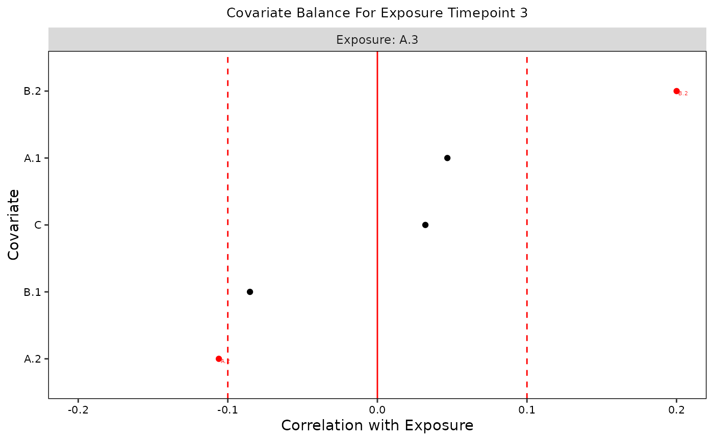
plot(b, t = "A.3")

plot(b, t = 3)


# Weighted
f <- createFormulas(obj, type = "short")
w <- createWeights(data = data, formulas = f)
bw <- assessBalance(data = data, weights = w)
print(bw)
#> 
#> +----------+-----------+---------------+------------+----------+
#> | exposure | covariate | std_bal_stats | bal_thresh | balanced |
#> +==========+===========+===============+============+==========+
#> | A.1      | C         | -0.1136       | 0.1        | 0        |
#> +----------+-----------+---------------+------------+----------+
#> | A.2      | C         | -0.0279       | 0.1        | 1        |
#> +----------+-----------+---------------+------------+----------+
#> | A.2      | B.1       | -0.0216       | 0.1        | 1        |
#> +----------+-----------+---------------+------------+----------+
#> | A.2      | A.1       |  0.1254       | 0.1        | 0        |
#> +----------+-----------+---------------+------------+----------+
#> | A.3      | C         | -0.0584       | 0.1        | 1        |
#> +----------+-----------+---------------+------------+----------+
#> | A.3      | B.1       | -0.0606       | 0.1        | 1        |
#> +----------+-----------+---------------+------------+----------+
#> | A.3      | B.2       | -0.0311       | 0.1        | 1        |
#> +----------+-----------+---------------+------------+----------+
#> | A.3      | A.1       | -0.0195       | 0.1        | 1        |
#> +----------+-----------+---------------+------------+----------+
#> | A.3      | A.2       | -0.1877       | 0.1        | 0        |
#> +----------+-----------+---------------+------------+----------+
#> 
#> Table: Balance Stats for All Exposure Time Points 
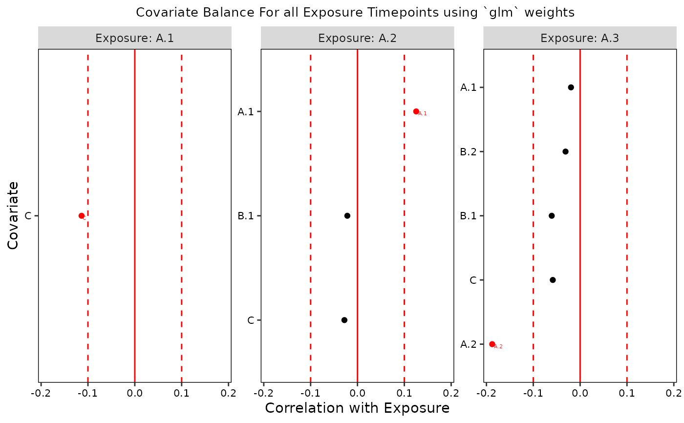
plot(bw)