Estimate, compare, and visualize exposure histories
Source:R/compareHistories.R
compareHistories.RdTakes fitted model output to created predicted values for user-specified histories (pooling for imputed data), before conducting contrast comparisons (pooling for imputed data), correcting for multiple comparisons, and then plotting results.
Usage
compareHistories(
  fit,
  hi_lo_cut,
  dose_level = "h",
  reference = NULL,
  comparison = NULL,
  outcome_level = NULL,
  mc_comp_method = "BH",
  verbose = FALSE,
  save.out = FALSE
)

# S3 method for class 'devMSM_comparisons'
print(x, save.out = FALSE, ...)

# S3 method for class 'devMSM_comparisons'
plot(
  x,
  colors = "Dark2",
  exp_lab = NULL,
  out_lab = NULL,
  save.out = FALSE,
  ...
)

# S3 method for class 'devMSM_comparisons'
summary(object, type = "comps", ...)
Arguments
- fit
list of model outputs from
fitModel()- hi_lo_cut
list of two numbers indicating quantile values that reflect high and low values, respectively, for continuous exposure
- dose_level
(optional) "l" or "h" indicating whether low or high doses should be tallied in tables and plots (default is high "h")
- reference
lists of one or more strings of "-"-separated "l" and "h" values indicative of a reference exposure history to which to compare comparison, required if comparison is supplied
- comparison
(optional) list of one or more strings of "-"-separated "l" and "h" values indicative of comparison history/histories to compare to reference, required if reference is supplied
- outcome_level
levels of a factor outcome within which the user wishes compare histories (default is all levels), history predictions and comparisons will be made within each outcome level.
- mc_comp_method
(optional) character abbreviation for multiple comparison correction method for stats::p.adjust, default is Benjamini-Hochburg ("BH")
- verbose
(optional) TRUE or FALSE indicator for printing output to console. default is FALSE.
- save.out
(optional) Either logical or a character string. If
TRUE, it will output the result to a default file name withinhome_dirset ininitMSM(). You can load the data withx <- readRDS(file). To use a non-default file name, specify a character string with the file name. It will save relative tohome_dir. There might be naming conflicts where two objects get saved to the same file. In these cases, users should specify a custom name. default is FALSE.- x
devMSM_histories object from
compareHistories()- ...
ignored
- colors
(optional) character specifying Brewer palette or list of colors (n(epochs)+1) for plotting (default is "Dark2" palette)
- exp_lab
(optional) character label for exposure variable in plots (default is variable name)
- out_lab
(optional) character label for outcome variable in plots (default is variable name)
- object
devMSM_histories object from
compareHistories()- type
Either "preds" or "comps" corresponding to the results of
marginaleffects::avg_predictions()at low and high dosages ormarginaleffects::avg_comparisons()respectively
Value
list containing two dataframes: preds with predictions from
marginaleffects::avg_predictions() containing average expected outcome
for different exposure histories and comps with contrasts from
marginaleffects::comparisons() comparing different exposure history
See also
marginaleffects::avg_predictions(),
https://cran.r-project.org/web/packages/marginaleffects/marginaleffects.pdf;
marginaleffects::hypotheses(),
https://cran.r-project.org/web/packages/marginaleffects/marginaleffects.pdf;
stats::p.adjust(),
https://www.rdocumentation.org/packages/stats/versions/3.6.2/topics/p.adjust;
Examples
library(devMSMs)
set.seed(123)
data <- data.frame(
ID = 1:50,
A.1 = rnorm(n = 50),
A.2 = rnorm(n = 50),
A.3 = rnorm(n = 50),
B.1 = rnorm(n = 50),
B.2 = rnorm(n = 50),
B.3 = rnorm(n = 50),
C = rnorm(n = 50),
D.3 = rnorm(n = 50)
)
obj <- initMSM(
data,
exposure = c("A.1", "A.2", "A.3"),
ti_conf = c("C"),
tv_conf = c("B.1", "B.2", "B.3", "D.3")
)
f <- createFormulas(obj, type = "short")
w <- createWeights(data = data, formulas = f)
fit <- fitModel(
data = data, weights = w,
outcome = "D.3", model = "m0"
)
comp <- compareHistories(
fit = fit,
hi_lo_cut = c(0.3, 0.6)
)
print(comp)
#> Summary of Exposure Main Effects:
#> USER ALERT: Out of the total of 50 individuals in the sample, below is the distribution of the 50 (100%) individuals that fall into 24 user-selected exposure histories (out of the 24 total) created from 30th and 60th percentile values for low and high levels of exposure-epoch A.1, A.2, A.3.
#> USER ALERT: Please inspect the distribution of the sample across the following exposure histories and ensure there is sufficient spread to avoid extrapolation and low precision:
#>
#> +---------------+---+
#> | epoch_history | n |
#> +===============+===+
#> | NA-NA-h | 2 |
#> +---------------+---+
#> | NA-NA-l | 1 |
#> +---------------+---+
#> | NA-h-NA | 2 |
#> +---------------+---+
#> | NA-h-h | 3 |
#> +---------------+---+
#> | NA-h-l | 2 |
#> +---------------+---+
#> | NA-l-NA | 1 |
#> +---------------+---+
#> | NA-l-h | 2 |
#> +---------------+---+
#> | NA-l-l | 2 |
#> +---------------+---+
#> | h-NA-NA | 2 |
#> +---------------+---+
#> | h-NA-h | 4 |
#> +---------------+---+
#> | h-NA-l | 1 |
#> +---------------+---+
#> | h-h-NA | 2 |
#> +---------------+---+
#> | h-h-h | 3 |
#> +---------------+---+
#> | h-h-l | 3 |
#> +---------------+---+
#> | h-l-NA | 1 |
#> +---------------+---+
#> | h-l-h | 2 |
#> +---------------+---+
#> | h-l-l | 2 |
#> +---------------+---+
#> | l-NA-NA | 3 |
#> +---------------+---+
#> | l-NA-l | 2 |
#> +---------------+---+
#> | l-h-NA | 2 |
#> +---------------+---+
#> | l-h-h | 1 |
#> +---------------+---+
#> | l-h-l | 2 |
#> +---------------+---+
#> | l-l-NA | 2 |
#> +---------------+---+
#> | l-l-h | 3 |
#> +---------------+---+
#>
#> Table: Summary of user-selected exposure histories based on exposure main effects A.1, A.2, A.3:
#>
#> Below are the pooled average predictions by user-specified history:
#> +-------+-------+------+--------+----------+-----------+----------+-----------+
#> | term | A.1 | A.2 | A.3 | estimate | std.error | conf.low | conf.high |
#> +=======+=======+======+========+==========+===========+==========+===========+
#> | l-l-l | -0.47 | -0.3 | -0.804 | -0.15 | 0.2 | -0.54 | 0.239 |
#> +-------+-------+------+--------+----------+-----------+----------+-----------+
#> | l-l-h | -0.47 | -0.3 | -0.051 | -0.064 | 0.2 | -0.47 | 0.338 |
#> +-------+-------+------+--------+----------+-----------+----------+-----------+
#> | l-h-l | -0.47 | 0.31 | -0.804 | -0.093 | 0.18 | -0.44 | 0.25 |
#> +-------+-------+------+--------+----------+-----------+----------+-----------+
#> | l-h-h | -0.47 | 0.31 | -0.051 | -0.007 | 0.19 | -0.37 | 0.357 |
#> +-------+-------+------+--------+----------+-----------+----------+-----------+
#> | h-l-l | 0.24 | -0.3 | -0.804 | -0.235 | 0.15 | -0.53 | 0.059 |
#> +-------+-------+------+--------+----------+-----------+----------+-----------+
#> | h-l-h | 0.24 | -0.3 | -0.051 | -0.149 | 0.15 | -0.45 | 0.154 |
#> +-------+-------+------+--------+----------+-----------+----------+-----------+
#> | h-h-l | 0.24 | 0.31 | -0.804 | -0.179 | 0.13 | -0.43 | 0.07 |
#> +-------+-------+------+--------+----------+-----------+----------+-----------+
#> | h-h-h | 0.24 | 0.31 | -0.051 | -0.093 | 0.14 | -0.36 | 0.176 |
#> +-------+-------+------+--------+----------+-----------+----------+-----------+
#>
#> Conducting multiple comparison correction for all pairings between comparison histories and each reference history using the BH method.
#>
#>
#> +-------------------+---------------+------------+-----------+-------------+------------+--------------+
#> | term | estimate | std.error | p.value | conf.low | conf.high | p.value_corr |
#> +===================+===============+============+===========+=============+============+==============+
#> | (l-l-h) - (l-l-l) | 0.0860245895 | 0.09323346 | 0.3561743 | -0.09670963 | 0.26875881 | 0.5955719 |
#> +-------------------+---------------+------------+-----------+-------------+------------+--------------+
#> | (l-h-l) - (l-l-l) | 0.0567671468 | 0.06804539 | 0.4041378 | -0.07659938 | 0.19013367 | 0.5955719 |
#> +-------------------+---------------+------------+-----------+-------------+------------+--------------+
#> | (l-h-h) - (l-l-l) | 0.1427917364 | 0.12113182 | 0.2384727 | -0.09462226 | 0.38020573 | 0.5955719 |
#> +-------------------+---------------+------------+-----------+-------------+------------+--------------+
#> | (h-l-l) - (l-l-l) | -0.0855518211 | 0.09515352 | 0.3686034 | -0.27204930 | 0.10094566 | 0.5955719 |
#> +-------------------+---------------+------------+-----------+-------------+------------+--------------+
#> | (h-l-h) - (l-l-l) | 0.0004727684 | 0.12853506 | 0.9970653 | -0.25145132 | 0.25239686 | 0.9970653 |
#> +-------------------+---------------+------------+-----------+-------------+------------+--------------+
#> | (h-h-l) - (l-l-l) | -0.0287846743 | 0.12605827 | 0.8193787 | -0.27585435 | 0.21828500 | 0.8824078 |
#> +-------------------+---------------+------------+-----------+-------------+------------+--------------+
#> | (h-h-h) - (l-l-l) | 0.0572399153 | 0.15718783 | 0.7157462 | -0.25084257 | 0.36532240 | 0.8824078 |
#> +-------------------+---------------+------------+-----------+-------------+------------+--------------+
#> | (l-l-l) - (l-l-h) | -0.0860245895 | 0.09323346 | 0.3561743 | -0.26875881 | 0.09670963 | 0.5955719 |
#> +-------------------+---------------+------------+-----------+-------------+------------+--------------+
#> | (l-h-l) - (l-l-h) | -0.0292574427 | 0.10941844 | 0.7891686 | -0.24371365 | 0.18519876 | 0.8824078 |
#> +-------------------+---------------+------------+-----------+-------------+------------+--------------+
#> | (l-h-h) - (l-l-h) | 0.0567671468 | 0.06804540 | 0.4041379 | -0.07659939 | 0.19013368 | 0.5955719 |
#> +-------------------+---------------+------------+-----------+-------------+------------+--------------+
#> | (h-l-l) - (l-l-h) | -0.1715764106 | 0.13773921 | 0.2128888 | -0.44154031 | 0.09838749 | 0.5955719 |
#> +-------------------+---------------+------------+-----------+-------------+------------+--------------+
#> | (h-l-h) - (l-l-h) | -0.0855518211 | 0.09515355 | 0.3686035 | -0.27204934 | 0.10094570 | 0.5955719 |
#> +-------------------+---------------+------------+-----------+-------------+------------+--------------+
#> | (h-h-l) - (l-l-h) | -0.1148092638 | 0.15639156 | 0.4628791 | -0.42133109 | 0.19171256 | 0.6480308 |
#> +-------------------+---------------+------------+-----------+-------------+------------+--------------+
#> | (h-h-h) - (l-l-h) | -0.0287846743 | 0.12605825 | 0.8193786 | -0.27585430 | 0.21828495 | 0.8824078 |
#> +-------------------+---------------+------------+-----------+-------------+------------+--------------+
#> | (l-l-l) - (l-h-l) | -0.0567671468 | 0.06804539 | 0.4041378 | -0.19013367 | 0.07659938 | 0.5955719 |
#> +-------------------+---------------+------------+-----------+-------------+------------+--------------+
#> | (l-l-h) - (l-h-l) | 0.0292574427 | 0.10941844 | 0.7891686 | -0.18519876 | 0.24371365 | 0.8824078 |
#> +-------------------+---------------+------------+-----------+-------------+------------+--------------+
#> | (l-h-h) - (l-h-l) | 0.0860245895 | 0.09323348 | 0.3561744 | -0.09670968 | 0.26875886 | 0.5955719 |
#> +-------------------+---------------+------------+-----------+-------------+------------+--------------+
#> | (h-l-l) - (l-h-l) | -0.1423189679 | 0.10713569 | 0.1840463 | -0.35230106 | 0.06766313 | 0.5955719 |
#> +-------------------+---------------+------------+-----------+-------------+------------+--------------+
#> | (h-l-h) - (l-h-l) | -0.0562943784 | 0.13264562 | 0.6712764 | -0.31627502 | 0.20368626 | 0.8824078 |
#> +-------------------+---------------+------------+-----------+-------------+------------+--------------+
#> | (h-h-l) - (l-h-l) | -0.0855518211 | 0.09515354 | 0.3686034 | -0.27204933 | 0.10094568 | 0.5955719 |
#> +-------------------+---------------+------------+-----------+-------------+------------+--------------+
#> | (h-h-h) - (l-h-l) | 0.0004727684 | 0.12853506 | 0.9970653 | -0.25145132 | 0.25239686 | 0.9970653 |
#> +-------------------+---------------+------------+-----------+-------------+------------+--------------+
#> | (l-l-l) - (l-h-h) | -0.1427917364 | 0.12113182 | 0.2384727 | -0.38020573 | 0.09462226 | 0.5955719 |
#> +-------------------+---------------+------------+-----------+-------------+------------+--------------+
#> | (l-l-h) - (l-h-h) | -0.0567671468 | 0.06804540 | 0.4041379 | -0.19013368 | 0.07659939 | 0.5955719 |
#> +-------------------+---------------+------------+-----------+-------------+------------+--------------+
#> | (l-h-l) - (l-h-h) | -0.0860245895 | 0.09323348 | 0.3561744 | -0.26875886 | 0.09670968 | 0.5955719 |
#> +-------------------+---------------+------------+-----------+-------------+------------+--------------+
#> | (h-l-l) - (l-h-h) | -0.2283435575 | 0.15081850 | 0.1300185 | -0.52394239 | 0.06725528 | 0.5955719 |
#> +-------------------+---------------+------------+-----------+-------------+------------+--------------+
#> | (h-l-h) - (l-h-h) | -0.1423189679 | 0.10713570 | 0.1840463 | -0.35230108 | 0.06766315 | 0.5955719 |
#> +-------------------+---------------+------------+-----------+-------------+------------+--------------+
#> | (h-h-l) - (l-h-h) | -0.1715764106 | 0.13773922 | 0.2128888 | -0.44154033 | 0.09838751 | 0.5955719 |
#> +-------------------+---------------+------------+-----------+-------------+------------+--------------+
#> | (h-h-h) - (l-h-h) | -0.0855518211 | 0.09515352 | 0.3686034 | -0.27204929 | 0.10094565 | 0.5955719 |
#> +-------------------+---------------+------------+-----------+-------------+------------+--------------+
#> | (l-l-l) - (h-l-l) | 0.0855518211 | 0.09515352 | 0.3686034 | -0.10094566 | 0.27204930 | 0.5955719 |
#> +-------------------+---------------+------------+-----------+-------------+------------+--------------+
#> | (l-l-h) - (h-l-l) | 0.1715764106 | 0.13773921 | 0.2128888 | -0.09838749 | 0.44154031 | 0.5955719 |
#> +-------------------+---------------+------------+-----------+-------------+------------+--------------+
#> | (l-h-l) - (h-l-l) | 0.1423189679 | 0.10713569 | 0.1840463 | -0.06766313 | 0.35230106 | 0.5955719 |
#> +-------------------+---------------+------------+-----------+-------------+------------+--------------+
#> | (l-h-h) - (h-l-l) | 0.2283435575 | 0.15081850 | 0.1300185 | -0.06725528 | 0.52394239 | 0.5955719 |
#> +-------------------+---------------+------------+-----------+-------------+------------+--------------+
#> | (h-l-h) - (h-l-l) | 0.0860245895 | 0.09323350 | 0.3561745 | -0.09670971 | 0.26875889 | 0.5955719 |
#> +-------------------+---------------+------------+-----------+-------------+------------+--------------+
#> | (h-h-l) - (h-l-l) | 0.0567671468 | 0.06804543 | 0.4041381 | -0.07659944 | 0.19013373 | 0.5955719 |
#> +-------------------+---------------+------------+-----------+-------------+------------+--------------+
#> | (h-h-h) - (h-l-l) | 0.1427917364 | 0.12113188 | 0.2384730 | -0.09462239 | 0.38020586 | 0.5955719 |
#> +-------------------+---------------+------------+-----------+-------------+------------+--------------+
#> | (l-l-l) - (h-l-h) | -0.0004727684 | 0.12853506 | 0.9970653 | -0.25239686 | 0.25145132 | 0.9970653 |
#> +-------------------+---------------+------------+-----------+-------------+------------+--------------+
#> | (l-l-h) - (h-l-h) | 0.0855518211 | 0.09515355 | 0.3686035 | -0.10094570 | 0.27204934 | 0.5955719 |
#> +-------------------+---------------+------------+-----------+-------------+------------+--------------+
#> | (l-h-l) - (h-l-h) | 0.0562943784 | 0.13264562 | 0.6712764 | -0.20368626 | 0.31627502 | 0.8824078 |
#> +-------------------+---------------+------------+-----------+-------------+------------+--------------+
#> | (l-h-h) - (h-l-h) | 0.1423189679 | 0.10713570 | 0.1840463 | -0.06766315 | 0.35230108 | 0.5955719 |
#> +-------------------+---------------+------------+-----------+-------------+------------+--------------+
#> | (h-l-l) - (h-l-h) | -0.0860245895 | 0.09323350 | 0.3561745 | -0.26875889 | 0.09670971 | 0.5955719 |
#> +-------------------+---------------+------------+-----------+-------------+------------+--------------+
#> | (h-h-l) - (h-l-h) | -0.0292574427 | 0.10941843 | 0.7891686 | -0.24371362 | 0.18519874 | 0.8824078 |
#> +-------------------+---------------+------------+-----------+-------------+------------+--------------+
#> | (h-h-h) - (h-l-h) | 0.0567671468 | 0.06804539 | 0.4041378 | -0.07659936 | 0.19013365 | 0.5955719 |
#> +-------------------+---------------+------------+-----------+-------------+------------+--------------+
#> | (l-l-l) - (h-h-l) | 0.0287846743 | 0.12605827 | 0.8193787 | -0.21828500 | 0.27585435 | 0.8824078 |
#> +-------------------+---------------+------------+-----------+-------------+------------+--------------+
#> | (l-l-h) - (h-h-l) | 0.1148092638 | 0.15639156 | 0.4628791 | -0.19171256 | 0.42133109 | 0.6480308 |
#> +-------------------+---------------+------------+-----------+-------------+------------+--------------+
#> | (l-h-l) - (h-h-l) | 0.0855518211 | 0.09515354 | 0.3686034 | -0.10094568 | 0.27204933 | 0.5955719 |
#> +-------------------+---------------+------------+-----------+-------------+------------+--------------+
#> | (l-h-h) - (h-h-l) | 0.1715764106 | 0.13773922 | 0.2128888 | -0.09838751 | 0.44154033 | 0.5955719 |
#> +-------------------+---------------+------------+-----------+-------------+------------+--------------+
#> | (h-l-l) - (h-h-l) | -0.0567671468 | 0.06804543 | 0.4041381 | -0.19013373 | 0.07659944 | 0.5955719 |
#> +-------------------+---------------+------------+-----------+-------------+------------+--------------+
#> | (h-l-h) - (h-h-l) | 0.0292574427 | 0.10941843 | 0.7891686 | -0.18519874 | 0.24371362 | 0.8824078 |
#> +-------------------+---------------+------------+-----------+-------------+------------+--------------+
#> | (h-h-h) - (h-h-l) | 0.0860245895 | 0.09323350 | 0.3561745 | -0.09670971 | 0.26875889 | 0.5955719 |
#> +-------------------+---------------+------------+-----------+-------------+------------+--------------+
#> | (l-l-l) - (h-h-h) | -0.0572399153 | 0.15718783 | 0.7157462 | -0.36532240 | 0.25084257 | 0.8824078 |
#> +-------------------+---------------+------------+-----------+-------------+------------+--------------+
#> | (l-l-h) - (h-h-h) | 0.0287846743 | 0.12605825 | 0.8193786 | -0.21828495 | 0.27585430 | 0.8824078 |
#> +-------------------+---------------+------------+-----------+-------------+------------+--------------+
#> | (l-h-l) - (h-h-h) | -0.0004727684 | 0.12853506 | 0.9970653 | -0.25239686 | 0.25145132 | 0.9970653 |
#> +-------------------+---------------+------------+-----------+-------------+------------+--------------+
#> | (l-h-h) - (h-h-h) | 0.0855518211 | 0.09515352 | 0.3686034 | -0.10094565 | 0.27204929 | 0.5955719 |
#> +-------------------+---------------+------------+-----------+-------------+------------+--------------+
#> | (h-l-l) - (h-h-h) | -0.1427917364 | 0.12113188 | 0.2384730 | -0.38020586 | 0.09462239 | 0.5955719 |
#> +-------------------+---------------+------------+-----------+-------------+------------+--------------+
#> | (h-l-h) - (h-h-h) | -0.0567671468 | 0.06804539 | 0.4041378 | -0.19013365 | 0.07659936 | 0.5955719 |
#> +-------------------+---------------+------------+-----------+-------------+------------+--------------+
#> | (h-h-l) - (h-h-h) | -0.0860245895 | 0.09323350 | 0.3561745 | -0.26875889 | 0.09670971 | 0.5955719 |
#> +-------------------+---------------+------------+-----------+-------------+------------+--------------+
plot(comp)
#> `height` was translated to `width`.
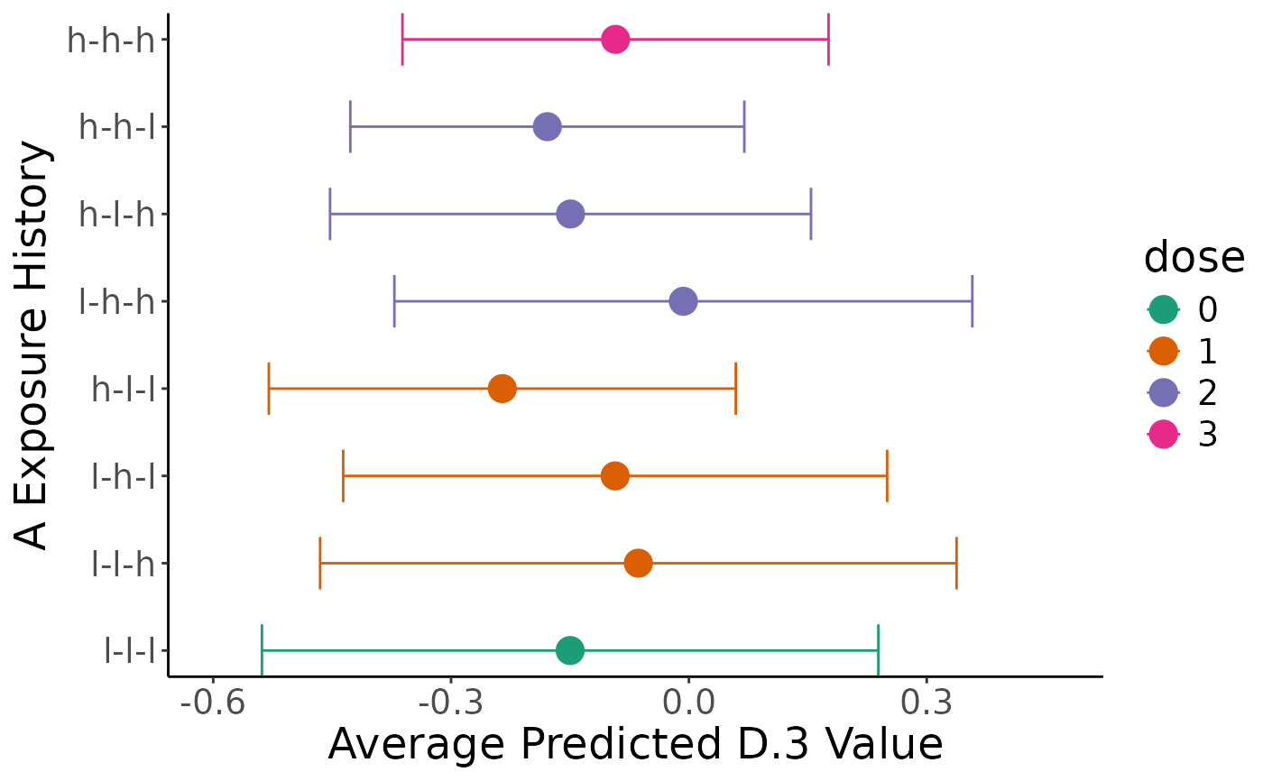 summary(comp, "preds")
#> term A.1 A.2 A.3 estimate std.error statistic
#> 1 l-l-l -0.4684962 -0.2971206 -0.80434443 -0.149799589 0.1983536 -0.75521497
#> 2 l-l-h -0.4684962 -0.2971206 -0.05134827 -0.063774999 0.2048054 -0.31139321
#> 3 l-h-l -0.4684962 0.3148300 -0.80434443 -0.093032442 0.1750306 -0.53152101
#> 4 l-h-h -0.4684962 0.3148300 -0.05134827 -0.007007852 0.1859760 -0.03768148
#> 5 h-l-l 0.2359494 -0.2971206 -0.80434443 -0.235351410 0.1502512 -1.56638593
#> 6 h-l-h 0.2359494 -0.2971206 -0.05134827 -0.149326820 0.1547615 -0.96488374
#> 7 h-h-l 0.2359494 0.3148300 -0.80434443 -0.178584263 0.1267806 -1.40860887
#> 8 h-h-h 0.2359494 0.3148300 -0.05134827 -0.092559673 0.1371105 -0.67507375
#> p.value s.value conf.low conf.high df dose
#> 1 0.4501200 1.15161839 -0.5385655 0.23896628 Inf 0
#> 2 0.7555017 0.40449307 -0.4651861 0.33763613 Inf 1
#> 3 0.5950578 0.74889832 -0.4360861 0.25002123 Inf 1
#> 4 0.9699416 0.04403015 -0.3715142 0.35749845 Inf 2
#> 5 0.1172583 3.09223810 -0.5298384 0.05913559 Inf 1
#> 6 0.3346030 1.57947751 -0.4526537 0.15400008 Inf 2
#> 7 0.1589509 2.65334732 -0.4270697 0.06990113 Inf 2
#> 8 0.4996289 1.00107114 -0.3612912 0.17617189 Inf 3
summary(comp, "comps")
#> term estimate std.error statistic p.value
#> 1 (l-l-h) - (l-l-l) 0.0860245895 0.09323346 0.922679369 0.3561743
#> 2 (l-h-l) - (l-l-l) 0.0567671468 0.06804539 0.834254060 0.4041378
#> 3 (l-h-h) - (l-l-l) 0.1427917364 0.12113182 1.178812803 0.2384727
#> 4 (h-l-l) - (l-l-l) -0.0855518211 0.09515352 -0.899092520 0.3686034
#> 5 (h-l-h) - (l-l-l) 0.0004727684 0.12853506 0.003678128 0.9970653
#> 6 (h-h-l) - (l-l-l) -0.0287846743 0.12605827 -0.228344191 0.8193787
#> 7 (h-h-h) - (l-l-l) 0.0572399153 0.15718783 0.364149793 0.7157462
#> 8 (l-l-l) - (l-l-h) -0.0860245895 0.09323346 -0.922679369 0.3561743
#> 9 (l-h-l) - (l-l-h) -0.0292574427 0.10941844 -0.267390415 0.7891686
#> 10 (l-h-h) - (l-l-h) 0.0567671468 0.06804540 0.834254004 0.4041379
#> 11 (h-l-l) - (l-l-h) -0.1715764106 0.13773921 -1.245661324 0.2128888
#> 12 (h-l-h) - (l-l-h) -0.0855518211 0.09515355 -0.899092314 0.3686035
#> 13 (h-h-l) - (l-l-h) -0.1148092638 0.15639156 -0.734114190 0.4628791
#> 14 (h-h-h) - (l-l-h) -0.0287846743 0.12605825 -0.228344235 0.8193786
#> 15 (l-l-l) - (l-h-l) -0.0567671468 0.06804539 -0.834254060 0.4041378
#> 16 (l-l-h) - (l-h-l) 0.0292574427 0.10941844 0.267390415 0.7891686
#> 17 (l-h-h) - (l-h-l) 0.0860245895 0.09323348 0.922679131 0.3561744
#> 18 (h-l-l) - (l-h-l) -0.1423189679 0.10713569 -1.328399218 0.1840463
#> 19 (h-l-h) - (l-h-l) -0.0562943784 0.13264562 -0.424396812 0.6712764
#> 20 (h-h-l) - (l-h-l) -0.0855518211 0.09515354 -0.899092399 0.3686034
#> 21 (h-h-h) - (l-h-l) 0.0004727684 0.12853506 0.003678128 0.9970653
#> 22 (l-l-l) - (l-h-h) -0.1427917364 0.12113182 -1.178812803 0.2384727
#> 23 (l-l-h) - (l-h-h) -0.0567671468 0.06804540 -0.834254004 0.4041379
#> 24 (l-h-l) - (l-h-h) -0.0860245895 0.09323348 -0.922679131 0.3561744
#> 25 (h-l-l) - (l-h-h) -0.2283435575 0.15081850 -1.514028790 0.1300185
#> 26 (h-l-h) - (l-h-h) -0.1423189679 0.10713570 -1.328399107 0.1840463
#> 27 (h-h-l) - (l-h-h) -0.1715764106 0.13773922 -1.245661218 0.2128888
#> 28 (h-h-h) - (l-h-h) -0.0855518211 0.09515352 -0.899092563 0.3686034
#> 29 (l-l-l) - (h-l-l) 0.0855518211 0.09515352 0.899092520 0.3686034
#> 30 (l-l-h) - (h-l-l) 0.1715764106 0.13773921 1.245661324 0.2128888
#> 31 (l-h-l) - (h-l-l) 0.1423189679 0.10713569 1.328399218 0.1840463
#> 32 (l-h-h) - (h-l-l) 0.2283435575 0.15081850 1.514028790 0.1300185
#> 33 (h-l-h) - (h-l-l) 0.0860245895 0.09323350 0.922678997 0.3561745
#> 34 (h-h-l) - (h-l-l) 0.0567671468 0.06804543 0.834253664 0.4041381
#> 35 (h-h-h) - (h-l-l) 0.1427917364 0.12113188 1.178812176 0.2384730
#> 36 (l-l-l) - (h-l-h) -0.0004727684 0.12853506 -0.003678128 0.9970653
#> 37 (l-l-h) - (h-l-h) 0.0855518211 0.09515355 0.899092314 0.3686035
#> 38 (l-h-l) - (h-l-h) 0.0562943784 0.13264562 0.424396812 0.6712764
#> 39 (l-h-h) - (h-l-h) 0.1423189679 0.10713570 1.328399107 0.1840463
#> 40 (h-l-l) - (h-l-h) -0.0860245895 0.09323350 -0.922678997 0.3561745
#> 41 (h-h-l) - (h-l-h) -0.0292574427 0.10941843 -0.267390446 0.7891686
#> 42 (h-h-h) - (h-l-h) 0.0567671468 0.06804539 0.834254172 0.4041378
#> 43 (l-l-l) - (h-h-l) 0.0287846743 0.12605827 0.228344191 0.8193787
#> 44 (l-l-h) - (h-h-l) 0.1148092638 0.15639156 0.734114190 0.4628791
#> 45 (l-h-l) - (h-h-l) 0.0855518211 0.09515354 0.899092399 0.3686034
#> 46 (l-h-h) - (h-h-l) 0.1715764106 0.13773922 1.245661218 0.2128888
#> 47 (h-l-l) - (h-h-l) -0.0567671468 0.06804543 -0.834253664 0.4041381
#> 48 (h-l-h) - (h-h-l) 0.0292574427 0.10941843 0.267390446 0.7891686
#> 49 (h-h-h) - (h-h-l) 0.0860245895 0.09323350 0.922678960 0.3561745
#> 50 (l-l-l) - (h-h-h) -0.0572399153 0.15718783 -0.364149793 0.7157462
#> 51 (l-l-h) - (h-h-h) 0.0287846743 0.12605825 0.228344235 0.8193786
#> 52 (l-h-l) - (h-h-h) -0.0004727684 0.12853506 -0.003678128 0.9970653
#> 53 (l-h-h) - (h-h-h) 0.0855518211 0.09515352 0.899092563 0.3686034
#> 54 (h-l-l) - (h-h-h) -0.1427917364 0.12113188 -1.178812176 0.2384730
#> 55 (h-l-h) - (h-h-h) -0.0567671468 0.06804539 -0.834254172 0.4041378
#> 56 (h-h-l) - (h-h-h) -0.0860245895 0.09323350 -0.922678960 0.3561745
#> s.value conf.low conf.high dose p.value_corr
#> 1 1.489344591 -0.09670963 0.26875881 1 - 0 0.5955719
#> 2 1.307080679 -0.07659938 0.19013367 1 - 0 0.5955719
#> 3 2.068103825 -0.09462226 0.38020573 2 - 0 0.5955719
#> 4 1.439858787 -0.27204930 0.10094566 1 - 0 0.5955719
#> 5 0.004240124 -0.25145132 0.25239686 2 - 0 0.9970653
#> 6 0.287397753 -0.27585435 0.21828500 2 - 0 0.8824078
#> 7 0.482480078 -0.25084257 0.36532240 3 - 0 0.8824078
#> 8 1.489344591 -0.26875881 0.09670963 0 - 1 0.5955719
#> 9 0.341594580 -0.24371365 0.18519876 1 - 1 0.8824078
#> 10 1.307080566 -0.07659939 0.19013368 2 - 1 0.5955719
#> 11 2.231828325 -0.44154031 0.09838749 1 - 1 0.5955719
#> 12 1.439858357 -0.27204934 0.10094570 2 - 1 0.5955719
#> 13 1.111292528 -0.42133109 0.19171256 2 - 1 0.6480308
#> 14 0.287397813 -0.27585430 0.21828495 3 - 1 0.8824078
#> 15 1.307080679 -0.19013367 0.07659938 0 - 1 0.5955719
#> 16 0.341594580 -0.18519876 0.24371365 1 - 1 0.8824078
#> 17 1.489344088 -0.09670968 0.26875886 2 - 1 0.5955719
#> 18 2.441859680 -0.35230106 0.06766313 1 - 1 0.5955719
#> 19 0.575021074 -0.31627502 0.20368626 2 - 1 0.8824078
#> 20 1.439858534 -0.27204933 0.10094568 2 - 1 0.5955719
#> 21 0.004240124 -0.25145132 0.25239686 3 - 1 0.9970653
#> 22 2.068103825 -0.38020573 0.09462226 0 - 2 0.5955719
#> 23 1.307080566 -0.19013368 0.07659939 1 - 2 0.5955719
#> 24 1.489344088 -0.26875886 0.09670968 1 - 2 0.5955719
#> 25 2.943210762 -0.52394239 0.06725528 1 - 2 0.5955719
#> 26 2.441859394 -0.35230108 0.06766315 2 - 2 0.5955719
#> 27 2.231828060 -0.44154033 0.09838751 2 - 2 0.5955719
#> 28 1.439858877 -0.27204929 0.10094565 3 - 2 0.5955719
#> 29 1.439858787 -0.10094566 0.27204930 0 - 1 0.5955719
#> 30 2.231828325 -0.09838749 0.44154031 1 - 1 0.5955719
#> 31 2.441859680 -0.06766313 0.35230106 1 - 1 0.5955719
#> 32 2.943210762 -0.06725528 0.52394239 2 - 1 0.5955719
#> 33 1.489343806 -0.09670971 0.26875889 2 - 1 0.5955719
#> 34 1.307079882 -0.07659944 0.19013373 2 - 1 0.5955719
#> 35 2.068102313 -0.09462239 0.38020586 3 - 1 0.5955719
#> 36 0.004240124 -0.25239686 0.25145132 0 - 2 0.9970653
#> 37 1.439858357 -0.10094570 0.27204934 1 - 2 0.5955719
#> 38 0.575021074 -0.20368626 0.31627502 1 - 2 0.8824078
#> 39 2.441859394 -0.06766315 0.35230108 2 - 2 0.5955719
#> 40 1.489343806 -0.26875889 0.09670971 1 - 2 0.5955719
#> 41 0.341594623 -0.24371362 0.18519874 2 - 2 0.8824078
#> 42 1.307080903 -0.07659936 0.19013365 3 - 2 0.5955719
#> 43 0.287397753 -0.21828500 0.27585435 0 - 2 0.8824078
#> 44 1.111292528 -0.19171256 0.42133109 1 - 2 0.6480308
#> 45 1.439858534 -0.10094568 0.27204933 1 - 2 0.5955719
#> 46 2.231828060 -0.09838751 0.44154033 2 - 2 0.5955719
#> 47 1.307079882 -0.19013373 0.07659944 1 - 2 0.5955719
#> 48 0.341594623 -0.18519874 0.24371362 2 - 2 0.8824078
#> 49 1.489343727 -0.09670971 0.26875889 3 - 2 0.5955719
#> 50 0.482480078 -0.36532240 0.25084257 0 - 3 0.8824078
#> 51 0.287397813 -0.21828495 0.27585430 1 - 3 0.8824078
#> 52 0.004240124 -0.25239686 0.25145132 1 - 3 0.9970653
#> 53 1.439858877 -0.10094565 0.27204929 2 - 3 0.5955719
#> 54 2.068102313 -0.38020586 0.09462239 1 - 3 0.5955719
#> 55 1.307080903 -0.19013365 0.07659936 2 - 3 0.5955719
#> 56 1.489343727 -0.26875889 0.09670971 2 - 3 0.5955719
comp2 <- compareHistories(
fit = fit,
hi_lo_cut = c(0.3, 0.6),
reference = "l-l-l",
comparison = c("h-h-h", "h-h-l")
)
print(comp2)
#> Summary of Exposure Main Effects:
#> Warning: There are no participants in your sample in the following histories: l-l-l.
#> Please revise your reference/comparison histories and/or the high/low cutoffs, if applicable.
#> USER ALERT: Out of the total of 50 individuals in the sample, below is the distribution of the 6 (12%) individuals that fall into 2 user-selected exposure histories (out of the 24 total) created from 30th and 60th percentile values for low and high levels of exposure-epoch A.1, A.2, A.3.
#> USER ALERT: Please inspect the distribution of the sample across the following exposure histories and ensure there is sufficient spread to avoid extrapolation and low precision:
#>
#> +---------------+---+
#> | epoch_history | n |
#> +===============+===+
#> | h-h-h | 3 |
#> +---------------+---+
#> | h-h-l | 3 |
#> +---------------+---+
#>
#> Table: Summary of user-selected exposure histories based on exposure main effects A.1, A.2, A.3:
#>
#> Below are the pooled average predictions by user-specified history:
#> +-------+-------+------+--------+----------+-----------+----------+-----------+
#> | term | A.1 | A.2 | A.3 | estimate | std.error | conf.low | conf.high |
#> +=======+=======+======+========+==========+===========+==========+===========+
#> | l-l-l | -0.47 | -0.3 | -0.804 | -0.15 | 0.2 | -0.54 | 0.24 |
#> +-------+-------+------+--------+----------+-----------+----------+-----------+
#> | h-h-l | 0.24 | 0.31 | -0.804 | -0.179 | 0.13 | -0.43 | 0.07 |
#> +-------+-------+------+--------+----------+-----------+----------+-----------+
#> | h-h-h | 0.24 | 0.31 | -0.051 | -0.093 | 0.14 | -0.36 | 0.18 |
#> +-------+-------+------+--------+----------+-----------+----------+-----------+
#>
#> Conducting multiple comparison correction for all pairings between comparison histories and each reference history using the BH method.
#>
#>
#> +-------------------+-------------+-----------+-----------+------------+-----------+--------------+
#> | term | estimate | std.error | p.value | conf.low | conf.high | p.value_corr |
#> +===================+=============+===========+===========+============+===========+==============+
#> | (h-h-h) - (l-l-l) | 0.05723992 | 0.1571878 | 0.7157462 | -0.2508426 | 0.3653224 | 0.8193787 |
#> +-------------------+-------------+-----------+-----------+------------+-----------+--------------+
#> | (h-h-l) - (l-l-l) | -0.02878467 | 0.1260583 | 0.8193787 | -0.2758543 | 0.2182850 | 0.8193787 |
#> +-------------------+-------------+-----------+-----------+------------+-----------+--------------+
plot(comp2)
#> `height` was translated to `width`.
summary(comp, "preds")
#> term A.1 A.2 A.3 estimate std.error statistic
#> 1 l-l-l -0.4684962 -0.2971206 -0.80434443 -0.149799589 0.1983536 -0.75521497
#> 2 l-l-h -0.4684962 -0.2971206 -0.05134827 -0.063774999 0.2048054 -0.31139321
#> 3 l-h-l -0.4684962 0.3148300 -0.80434443 -0.093032442 0.1750306 -0.53152101
#> 4 l-h-h -0.4684962 0.3148300 -0.05134827 -0.007007852 0.1859760 -0.03768148
#> 5 h-l-l 0.2359494 -0.2971206 -0.80434443 -0.235351410 0.1502512 -1.56638593
#> 6 h-l-h 0.2359494 -0.2971206 -0.05134827 -0.149326820 0.1547615 -0.96488374
#> 7 h-h-l 0.2359494 0.3148300 -0.80434443 -0.178584263 0.1267806 -1.40860887
#> 8 h-h-h 0.2359494 0.3148300 -0.05134827 -0.092559673 0.1371105 -0.67507375
#> p.value s.value conf.low conf.high df dose
#> 1 0.4501200 1.15161839 -0.5385655 0.23896628 Inf 0
#> 2 0.7555017 0.40449307 -0.4651861 0.33763613 Inf 1
#> 3 0.5950578 0.74889832 -0.4360861 0.25002123 Inf 1
#> 4 0.9699416 0.04403015 -0.3715142 0.35749845 Inf 2
#> 5 0.1172583 3.09223810 -0.5298384 0.05913559 Inf 1
#> 6 0.3346030 1.57947751 -0.4526537 0.15400008 Inf 2
#> 7 0.1589509 2.65334732 -0.4270697 0.06990113 Inf 2
#> 8 0.4996289 1.00107114 -0.3612912 0.17617189 Inf 3
summary(comp, "comps")
#> term estimate std.error statistic p.value
#> 1 (l-l-h) - (l-l-l) 0.0860245895 0.09323346 0.922679369 0.3561743
#> 2 (l-h-l) - (l-l-l) 0.0567671468 0.06804539 0.834254060 0.4041378
#> 3 (l-h-h) - (l-l-l) 0.1427917364 0.12113182 1.178812803 0.2384727
#> 4 (h-l-l) - (l-l-l) -0.0855518211 0.09515352 -0.899092520 0.3686034
#> 5 (h-l-h) - (l-l-l) 0.0004727684 0.12853506 0.003678128 0.9970653
#> 6 (h-h-l) - (l-l-l) -0.0287846743 0.12605827 -0.228344191 0.8193787
#> 7 (h-h-h) - (l-l-l) 0.0572399153 0.15718783 0.364149793 0.7157462
#> 8 (l-l-l) - (l-l-h) -0.0860245895 0.09323346 -0.922679369 0.3561743
#> 9 (l-h-l) - (l-l-h) -0.0292574427 0.10941844 -0.267390415 0.7891686
#> 10 (l-h-h) - (l-l-h) 0.0567671468 0.06804540 0.834254004 0.4041379
#> 11 (h-l-l) - (l-l-h) -0.1715764106 0.13773921 -1.245661324 0.2128888
#> 12 (h-l-h) - (l-l-h) -0.0855518211 0.09515355 -0.899092314 0.3686035
#> 13 (h-h-l) - (l-l-h) -0.1148092638 0.15639156 -0.734114190 0.4628791
#> 14 (h-h-h) - (l-l-h) -0.0287846743 0.12605825 -0.228344235 0.8193786
#> 15 (l-l-l) - (l-h-l) -0.0567671468 0.06804539 -0.834254060 0.4041378
#> 16 (l-l-h) - (l-h-l) 0.0292574427 0.10941844 0.267390415 0.7891686
#> 17 (l-h-h) - (l-h-l) 0.0860245895 0.09323348 0.922679131 0.3561744
#> 18 (h-l-l) - (l-h-l) -0.1423189679 0.10713569 -1.328399218 0.1840463
#> 19 (h-l-h) - (l-h-l) -0.0562943784 0.13264562 -0.424396812 0.6712764
#> 20 (h-h-l) - (l-h-l) -0.0855518211 0.09515354 -0.899092399 0.3686034
#> 21 (h-h-h) - (l-h-l) 0.0004727684 0.12853506 0.003678128 0.9970653
#> 22 (l-l-l) - (l-h-h) -0.1427917364 0.12113182 -1.178812803 0.2384727
#> 23 (l-l-h) - (l-h-h) -0.0567671468 0.06804540 -0.834254004 0.4041379
#> 24 (l-h-l) - (l-h-h) -0.0860245895 0.09323348 -0.922679131 0.3561744
#> 25 (h-l-l) - (l-h-h) -0.2283435575 0.15081850 -1.514028790 0.1300185
#> 26 (h-l-h) - (l-h-h) -0.1423189679 0.10713570 -1.328399107 0.1840463
#> 27 (h-h-l) - (l-h-h) -0.1715764106 0.13773922 -1.245661218 0.2128888
#> 28 (h-h-h) - (l-h-h) -0.0855518211 0.09515352 -0.899092563 0.3686034
#> 29 (l-l-l) - (h-l-l) 0.0855518211 0.09515352 0.899092520 0.3686034
#> 30 (l-l-h) - (h-l-l) 0.1715764106 0.13773921 1.245661324 0.2128888
#> 31 (l-h-l) - (h-l-l) 0.1423189679 0.10713569 1.328399218 0.1840463
#> 32 (l-h-h) - (h-l-l) 0.2283435575 0.15081850 1.514028790 0.1300185
#> 33 (h-l-h) - (h-l-l) 0.0860245895 0.09323350 0.922678997 0.3561745
#> 34 (h-h-l) - (h-l-l) 0.0567671468 0.06804543 0.834253664 0.4041381
#> 35 (h-h-h) - (h-l-l) 0.1427917364 0.12113188 1.178812176 0.2384730
#> 36 (l-l-l) - (h-l-h) -0.0004727684 0.12853506 -0.003678128 0.9970653
#> 37 (l-l-h) - (h-l-h) 0.0855518211 0.09515355 0.899092314 0.3686035
#> 38 (l-h-l) - (h-l-h) 0.0562943784 0.13264562 0.424396812 0.6712764
#> 39 (l-h-h) - (h-l-h) 0.1423189679 0.10713570 1.328399107 0.1840463
#> 40 (h-l-l) - (h-l-h) -0.0860245895 0.09323350 -0.922678997 0.3561745
#> 41 (h-h-l) - (h-l-h) -0.0292574427 0.10941843 -0.267390446 0.7891686
#> 42 (h-h-h) - (h-l-h) 0.0567671468 0.06804539 0.834254172 0.4041378
#> 43 (l-l-l) - (h-h-l) 0.0287846743 0.12605827 0.228344191 0.8193787
#> 44 (l-l-h) - (h-h-l) 0.1148092638 0.15639156 0.734114190 0.4628791
#> 45 (l-h-l) - (h-h-l) 0.0855518211 0.09515354 0.899092399 0.3686034
#> 46 (l-h-h) - (h-h-l) 0.1715764106 0.13773922 1.245661218 0.2128888
#> 47 (h-l-l) - (h-h-l) -0.0567671468 0.06804543 -0.834253664 0.4041381
#> 48 (h-l-h) - (h-h-l) 0.0292574427 0.10941843 0.267390446 0.7891686
#> 49 (h-h-h) - (h-h-l) 0.0860245895 0.09323350 0.922678960 0.3561745
#> 50 (l-l-l) - (h-h-h) -0.0572399153 0.15718783 -0.364149793 0.7157462
#> 51 (l-l-h) - (h-h-h) 0.0287846743 0.12605825 0.228344235 0.8193786
#> 52 (l-h-l) - (h-h-h) -0.0004727684 0.12853506 -0.003678128 0.9970653
#> 53 (l-h-h) - (h-h-h) 0.0855518211 0.09515352 0.899092563 0.3686034
#> 54 (h-l-l) - (h-h-h) -0.1427917364 0.12113188 -1.178812176 0.2384730
#> 55 (h-l-h) - (h-h-h) -0.0567671468 0.06804539 -0.834254172 0.4041378
#> 56 (h-h-l) - (h-h-h) -0.0860245895 0.09323350 -0.922678960 0.3561745
#> s.value conf.low conf.high dose p.value_corr
#> 1 1.489344591 -0.09670963 0.26875881 1 - 0 0.5955719
#> 2 1.307080679 -0.07659938 0.19013367 1 - 0 0.5955719
#> 3 2.068103825 -0.09462226 0.38020573 2 - 0 0.5955719
#> 4 1.439858787 -0.27204930 0.10094566 1 - 0 0.5955719
#> 5 0.004240124 -0.25145132 0.25239686 2 - 0 0.9970653
#> 6 0.287397753 -0.27585435 0.21828500 2 - 0 0.8824078
#> 7 0.482480078 -0.25084257 0.36532240 3 - 0 0.8824078
#> 8 1.489344591 -0.26875881 0.09670963 0 - 1 0.5955719
#> 9 0.341594580 -0.24371365 0.18519876 1 - 1 0.8824078
#> 10 1.307080566 -0.07659939 0.19013368 2 - 1 0.5955719
#> 11 2.231828325 -0.44154031 0.09838749 1 - 1 0.5955719
#> 12 1.439858357 -0.27204934 0.10094570 2 - 1 0.5955719
#> 13 1.111292528 -0.42133109 0.19171256 2 - 1 0.6480308
#> 14 0.287397813 -0.27585430 0.21828495 3 - 1 0.8824078
#> 15 1.307080679 -0.19013367 0.07659938 0 - 1 0.5955719
#> 16 0.341594580 -0.18519876 0.24371365 1 - 1 0.8824078
#> 17 1.489344088 -0.09670968 0.26875886 2 - 1 0.5955719
#> 18 2.441859680 -0.35230106 0.06766313 1 - 1 0.5955719
#> 19 0.575021074 -0.31627502 0.20368626 2 - 1 0.8824078
#> 20 1.439858534 -0.27204933 0.10094568 2 - 1 0.5955719
#> 21 0.004240124 -0.25145132 0.25239686 3 - 1 0.9970653
#> 22 2.068103825 -0.38020573 0.09462226 0 - 2 0.5955719
#> 23 1.307080566 -0.19013368 0.07659939 1 - 2 0.5955719
#> 24 1.489344088 -0.26875886 0.09670968 1 - 2 0.5955719
#> 25 2.943210762 -0.52394239 0.06725528 1 - 2 0.5955719
#> 26 2.441859394 -0.35230108 0.06766315 2 - 2 0.5955719
#> 27 2.231828060 -0.44154033 0.09838751 2 - 2 0.5955719
#> 28 1.439858877 -0.27204929 0.10094565 3 - 2 0.5955719
#> 29 1.439858787 -0.10094566 0.27204930 0 - 1 0.5955719
#> 30 2.231828325 -0.09838749 0.44154031 1 - 1 0.5955719
#> 31 2.441859680 -0.06766313 0.35230106 1 - 1 0.5955719
#> 32 2.943210762 -0.06725528 0.52394239 2 - 1 0.5955719
#> 33 1.489343806 -0.09670971 0.26875889 2 - 1 0.5955719
#> 34 1.307079882 -0.07659944 0.19013373 2 - 1 0.5955719
#> 35 2.068102313 -0.09462239 0.38020586 3 - 1 0.5955719
#> 36 0.004240124 -0.25239686 0.25145132 0 - 2 0.9970653
#> 37 1.439858357 -0.10094570 0.27204934 1 - 2 0.5955719
#> 38 0.575021074 -0.20368626 0.31627502 1 - 2 0.8824078
#> 39 2.441859394 -0.06766315 0.35230108 2 - 2 0.5955719
#> 40 1.489343806 -0.26875889 0.09670971 1 - 2 0.5955719
#> 41 0.341594623 -0.24371362 0.18519874 2 - 2 0.8824078
#> 42 1.307080903 -0.07659936 0.19013365 3 - 2 0.5955719
#> 43 0.287397753 -0.21828500 0.27585435 0 - 2 0.8824078
#> 44 1.111292528 -0.19171256 0.42133109 1 - 2 0.6480308
#> 45 1.439858534 -0.10094568 0.27204933 1 - 2 0.5955719
#> 46 2.231828060 -0.09838751 0.44154033 2 - 2 0.5955719
#> 47 1.307079882 -0.19013373 0.07659944 1 - 2 0.5955719
#> 48 0.341594623 -0.18519874 0.24371362 2 - 2 0.8824078
#> 49 1.489343727 -0.09670971 0.26875889 3 - 2 0.5955719
#> 50 0.482480078 -0.36532240 0.25084257 0 - 3 0.8824078
#> 51 0.287397813 -0.21828495 0.27585430 1 - 3 0.8824078
#> 52 0.004240124 -0.25239686 0.25145132 1 - 3 0.9970653
#> 53 1.439858877 -0.10094565 0.27204929 2 - 3 0.5955719
#> 54 2.068102313 -0.38020586 0.09462239 1 - 3 0.5955719
#> 55 1.307080903 -0.19013365 0.07659936 2 - 3 0.5955719
#> 56 1.489343727 -0.26875889 0.09670971 2 - 3 0.5955719
comp2 <- compareHistories(
fit = fit,
hi_lo_cut = c(0.3, 0.6),
reference = "l-l-l",
comparison = c("h-h-h", "h-h-l")
)
print(comp2)
#> Summary of Exposure Main Effects:
#> Warning: There are no participants in your sample in the following histories: l-l-l.
#> Please revise your reference/comparison histories and/or the high/low cutoffs, if applicable.
#> USER ALERT: Out of the total of 50 individuals in the sample, below is the distribution of the 6 (12%) individuals that fall into 2 user-selected exposure histories (out of the 24 total) created from 30th and 60th percentile values for low and high levels of exposure-epoch A.1, A.2, A.3.
#> USER ALERT: Please inspect the distribution of the sample across the following exposure histories and ensure there is sufficient spread to avoid extrapolation and low precision:
#>
#> +---------------+---+
#> | epoch_history | n |
#> +===============+===+
#> | h-h-h | 3 |
#> +---------------+---+
#> | h-h-l | 3 |
#> +---------------+---+
#>
#> Table: Summary of user-selected exposure histories based on exposure main effects A.1, A.2, A.3:
#>
#> Below are the pooled average predictions by user-specified history:
#> +-------+-------+------+--------+----------+-----------+----------+-----------+
#> | term | A.1 | A.2 | A.3 | estimate | std.error | conf.low | conf.high |
#> +=======+=======+======+========+==========+===========+==========+===========+
#> | l-l-l | -0.47 | -0.3 | -0.804 | -0.15 | 0.2 | -0.54 | 0.24 |
#> +-------+-------+------+--------+----------+-----------+----------+-----------+
#> | h-h-l | 0.24 | 0.31 | -0.804 | -0.179 | 0.13 | -0.43 | 0.07 |
#> +-------+-------+------+--------+----------+-----------+----------+-----------+
#> | h-h-h | 0.24 | 0.31 | -0.051 | -0.093 | 0.14 | -0.36 | 0.18 |
#> +-------+-------+------+--------+----------+-----------+----------+-----------+
#>
#> Conducting multiple comparison correction for all pairings between comparison histories and each reference history using the BH method.
#>
#>
#> +-------------------+-------------+-----------+-----------+------------+-----------+--------------+
#> | term | estimate | std.error | p.value | conf.low | conf.high | p.value_corr |
#> +===================+=============+===========+===========+============+===========+==============+
#> | (h-h-h) - (l-l-l) | 0.05723992 | 0.1571878 | 0.7157462 | -0.2508426 | 0.3653224 | 0.8193787 |
#> +-------------------+-------------+-----------+-----------+------------+-----------+--------------+
#> | (h-h-l) - (l-l-l) | -0.02878467 | 0.1260583 | 0.8193787 | -0.2758543 | 0.2182850 | 0.8193787 |
#> +-------------------+-------------+-----------+-----------+------------+-----------+--------------+
plot(comp2)
#> `height` was translated to `width`.
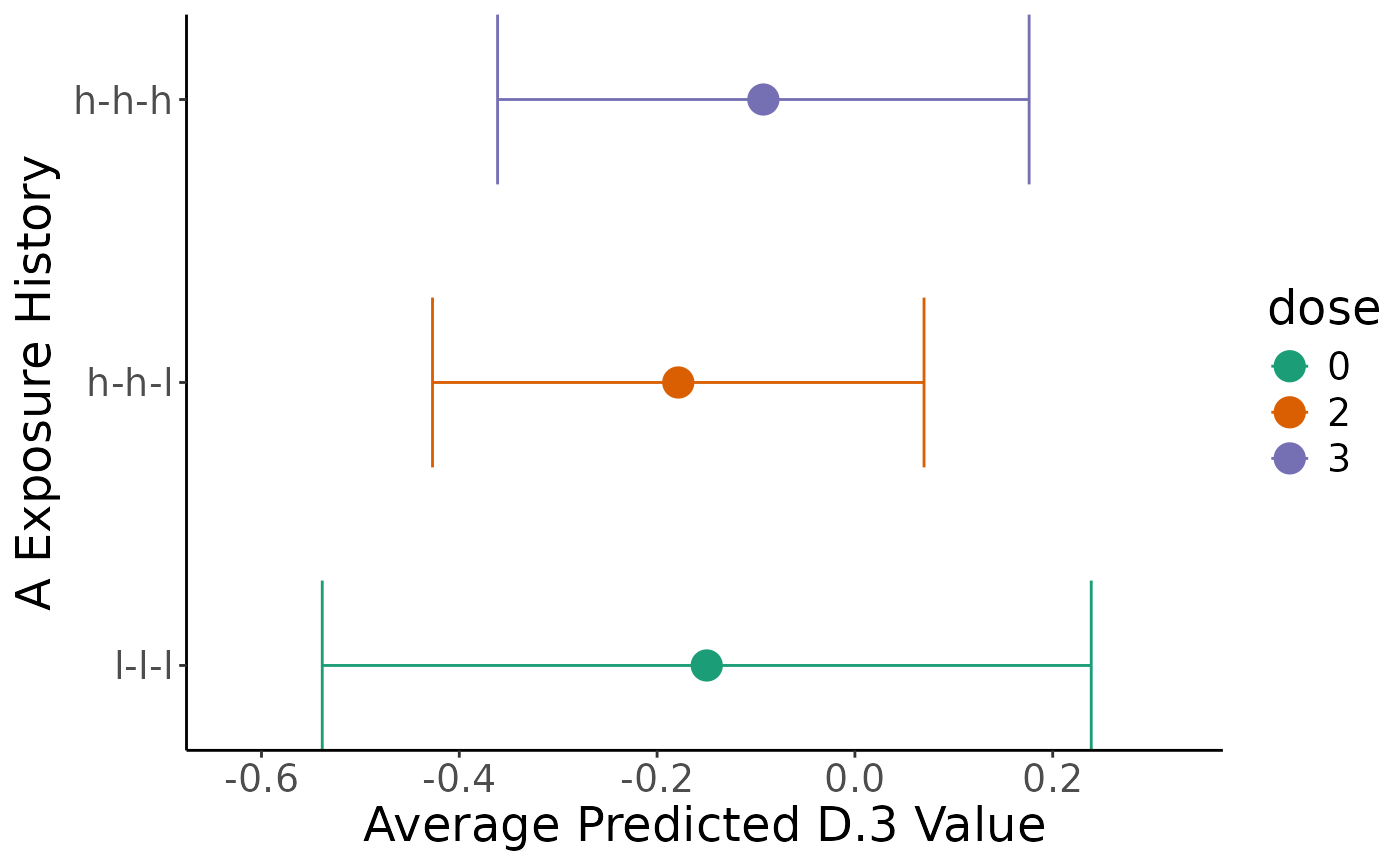 summary(comp2, "preds")
#> term A.1 A.2 A.3 estimate std.error statistic
#> 1 l-l-l -0.4684962 -0.2971206 -0.80434443 -0.14979959 0.1983536 -0.7552150
#> 7 h-h-l 0.2359494 0.3148300 -0.80434443 -0.17858426 0.1267806 -1.4086089
#> 8 h-h-h 0.2359494 0.3148300 -0.05134827 -0.09255967 0.1371105 -0.6750738
#> p.value s.value conf.low conf.high df dose
#> 1 0.4501200 1.151618 -0.5385655 0.23896628 Inf 0
#> 7 0.1589509 2.653347 -0.4270697 0.06990113 Inf 2
#> 8 0.4996289 1.001071 -0.3612912 0.17617189 Inf 3
summary(comp2, "comps")
#> term estimate std.error statistic p.value s.value
#> 1 (h-h-h) - (l-l-l) 0.05723992 0.1571878 0.3641498 0.7157462 0.4824801
#> 2 (h-h-l) - (l-l-l) -0.02878467 0.1260583 -0.2283442 0.8193787 0.2873978
#> conf.low conf.high dose p.value_corr
#> 1 -0.2508426 0.3653224 3 - 0 0.8193787
#> 2 -0.2758543 0.2182850 2 - 0 0.8193787
summary(comp2, "preds")
#> term A.1 A.2 A.3 estimate std.error statistic
#> 1 l-l-l -0.4684962 -0.2971206 -0.80434443 -0.14979959 0.1983536 -0.7552150
#> 7 h-h-l 0.2359494 0.3148300 -0.80434443 -0.17858426 0.1267806 -1.4086089
#> 8 h-h-h 0.2359494 0.3148300 -0.05134827 -0.09255967 0.1371105 -0.6750738
#> p.value s.value conf.low conf.high df dose
#> 1 0.4501200 1.151618 -0.5385655 0.23896628 Inf 0
#> 7 0.1589509 2.653347 -0.4270697 0.06990113 Inf 2
#> 8 0.4996289 1.001071 -0.3612912 0.17617189 Inf 3
summary(comp2, "comps")
#> term estimate std.error statistic p.value s.value
#> 1 (h-h-h) - (l-l-l) 0.05723992 0.1571878 0.3641498 0.7157462 0.4824801
#> 2 (h-h-l) - (l-l-l) -0.02878467 0.1260583 -0.2283442 0.8193787 0.2873978
#> conf.low conf.high dose p.value_corr
#> 1 -0.2508426 0.3653224 3 - 0 0.8193787
#> 2 -0.2758543 0.2182850 2 - 0 0.8193787