Trims IPTW balancing weights with heavy right tails by populating all weight values above a given quantile with the weight value of that quantile.
Arguments
- weights
list of IPTW weights output from
createWeights()- at
numeric; either the quantile of the weights above which weights are to be trimmed. A single number between .5 and 1, or the number of weights to be trimmed (e.g.,at = 3for the top 3 weights to be set to the 4th largest weight).- lower
logical; whether also to trim at the lower quantile (e.g., forat = .9, trimming at both .1 and .9, or forat = 3, trimming the top and bottom 3 weights). Default isFALSEto only trim the higher weights.- verbose
(optional) TRUE or FALSE indicator for printing output to console. default is FALSE.
- save.out
(optional) Either logical or a character string. If
TRUE, it will output the result to a default file name withinhome_dirset ininitMSM(). You can load the data withx <- readRDS(file). To use a non-default file name, specify a character string with the file name. It will save relative tohome_dir. There might be naming conflicts where two objects get saved to the same file. In these cases, users should specify a custom name. default is FALSE.
Value
a list containing WeightIt::weightitMSM() output. It is the length
of the number of datasets (1 for a data.frame or the number of imputed datasets).
See also
WeightIt::trim(),
https://search.r-project.org/CRAN/refmans/WeightIt/html/trim.html which
this function wraps
Examples
library(devMSMs)
data <- data.frame(
  ID = 1:50,
  A.1 = rnorm(n = 50),
  A.2 = rnorm(n = 50),
  A.3 = rnorm(n = 50),
  B.1 = rnorm(n = 50),
  B.2 = rnorm(n = 50),
  B.3 = rnorm(n = 50),
  C = rnorm(n = 50),
  D.3 = rnorm(n = 50)
)
obj <- initMSM(
  data,
  exposure = c("A.1", "A.2", "A.3"),
  ti_conf = c("C"),
  tv_conf = c("B.1", "B.2", "B.3", "D.3")
)
f <- createFormulas(obj, type = "short")

w <- createWeights(data = data, formulas = f)
tw <- trimWeights(w, at = 0.975)
print(tw)
#>
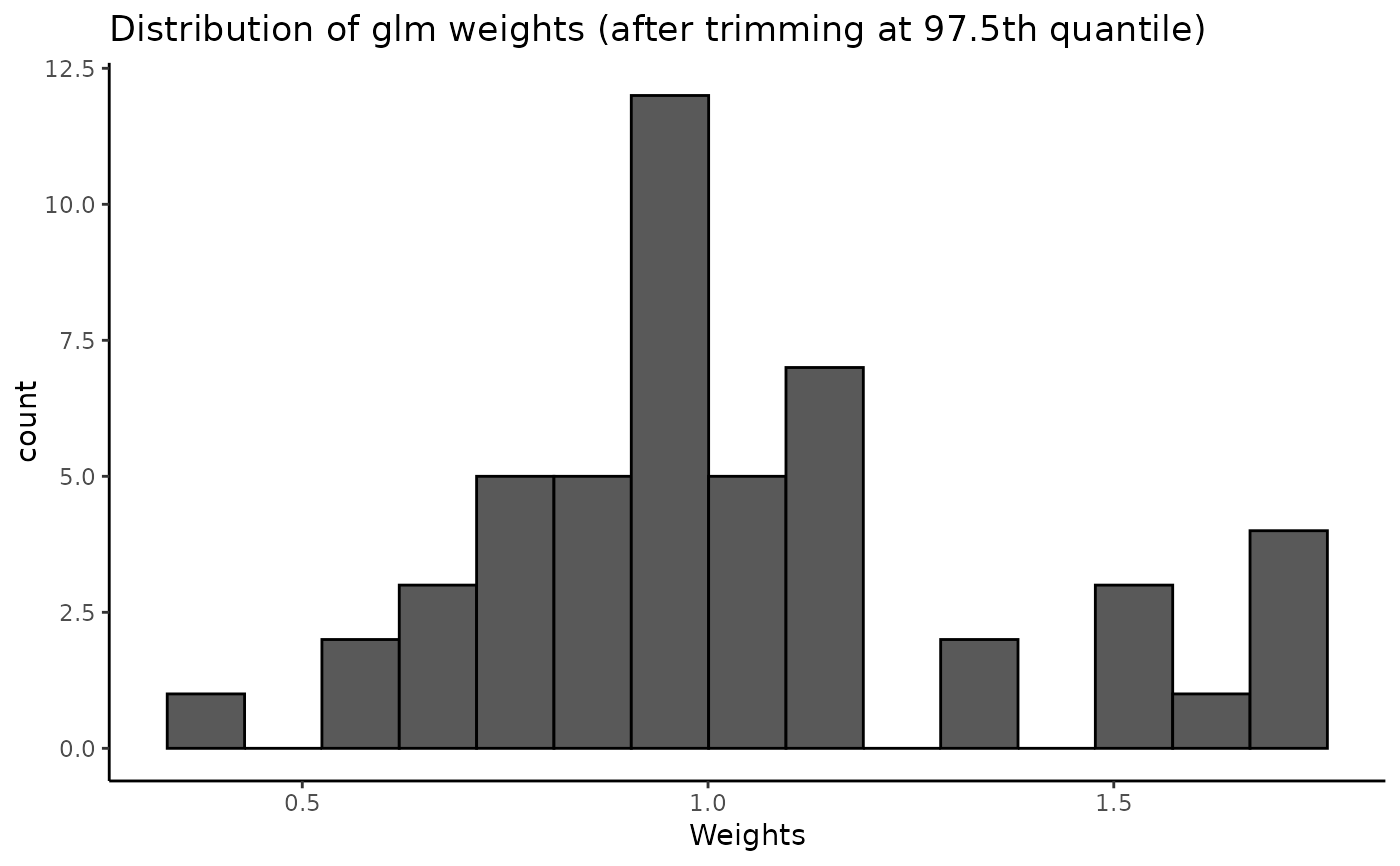
#> For the `glm` weighting method, after trimming at 97.5th quantile, the median weight value is 0.98 (SD = 0.7; range = 0.11-4).
plot(tw)


trimWeights(w, at = 0.975, lower = TRUE)
#>
#> For the `glm` weighting method, after trimming between 2.5th and 97.5th quantiles, the median weight value is 0.98 (SD = 0.7; range = 0.11-4).